The Preparation of Superconducting Qubits

The majority of new methods used for building a large-scale quantum computer often find it difficult to control a vast number of qubits.

In particular, systems built on superconducting circuits require a huge number of microwave control channels and readout channels. [1] Conventional solutions having low channel count AWGs are not conducive with regards to size and cost, and also have limitations with respect to the complexity and synchronization of systems.

UHFQA Quantum Analyzer and HDAWG Arbitrary Waveform Generator from Zurich Instrument offers the possibility of a highly integrated platform for both readout and control, ready to scale up the number of qubits. This article presents how Zurich Instruments hardware can be advantageously used to control a 4-qubit experiment, as implemented in the Quantum Device Lab at ETH Zurich, Switzerland.

Sample and Setup

Single qubit operations and the related control hardware are initially taken into account and then the multi-qubit case is considered. In superconducting circuit technology, a qubit contains a non-linear LC circuit, similar to the structure depicted in Figure 1. [2, 3]

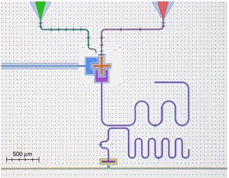
Figure 1. Colored microscope picture of a qubit unit cell: charge-line (green), flux-line (red), qubit island (orange), coupling resonator (blue), readout circuitry with Purcell-filter (violet) and feed-line (yellow). The chip substrate is Silicon with Niobium as a superconducting metal layer. [3]

For this LC circuit, the capacitance is given by a cross-shaped metal island, which is etched out of the superconducting metal plane (indicated in orange color). Along with a loop of a pair of tiny Josephson-junctions linked to this island, a weakly non-linear resonator is produced. The total qubit inductance relies on the magnetic flux via this loop. Therefore, the qubit resonance frequency can be modified by changing the local magnetic field via the current carried by the flux-line (indicated in red color) shorted nearby.

The resonator’s anharmonicity causes the energy levels to spread unevenly. To address individual energy transitions, the circuit is stimulated with a resonant microwave tone via the capacitively coupled charge line (indicated in green color). Manipulation of qubit states is done by modulating this resonant microwave tone with short microwave pulses offered by one channel pair of the HDAWG, up-converted to microwave frequency through an IQ mixer. [4]

The sample, indicated in Figure 1, is installed in a dilution refrigerator to give a well-isolated low-temperature environment that protects the circuit’s quantum properties.

In order to achieve qubit readout, a transmission-line resonator is dispersively coupled to the qubit and this readout circuitry is driven with a resonant tone (indicated in violet color). [5] Based on the qubit state, this readout resonator will currently have a marginally different frequency response, which is assessed by the UHFQA through the yellow-colored feedline.

To suppress further decay of the qubit state through the readout circuitry, a second transmission-line resonator or Purcell-filter is also placed in between the feedline and readout resonator. [6] In addition, multiple qubits can be read out simultaneously by using a single common feedline for all readout circuits and executing a frequency multiplexed pulse scheme. [7] For this purpose, the UHFQA generates a tone containing all readout resonator frequencies and this is later inspected to differentiate the individual qubit states.

In general, quantum computing applications need interactions between qubits. In this case, a coupling resonator (indicated in blue color) is used to link two adjacent qubits that are temporarily brought into resonance by modifying the DC current via the respective flux-line. Standard coupling strengths cause the qubit states to exchange within hundreds of nanoseconds. As illustrated in Figure 2, a four-channel HDAWG can provide high-time resolution signals needed at the flux-line inputs.

Figure 2. Simplified sketch of the 4-qubit experiment. Qubit readout is carried out by the UHFQA, qubit state manipulation by HDAWG 1 and qubit-qubit coupling is activated by HDAWG 2. For simplicity the local-oscillators, microwave amplifiers, filters and attenuators are not included in this sketch; see [4] for further details.

Measurements

Single Qubit Characterization

For a successful set up of a qubit experiment, all elements have to be initially characterized and all operations have to be calibrated. As a preliminary step, the UHFQA Quantum Analyzer is used to perform a spectroscopy over the common feedline. This is done to establish the exact resonance frequencies of all four readout resonators. For this type of measurement, the frequency of a continuous wave tone (CW) at the feedline input is swept and the amplitude of the transmitted signal is evaluated with the UHFQA Quantum Analyzer.

The frequencies of the qubits are then asserted by tracking the dispersive frequency shift in the readout circuitry using a two-tone microwave spectroscopy. The first tone in the spectroscopy drives the readout resonator and is fixed in frequency. The second tone is applied via the qubit charge line and is swept until the qubit’s resonant excitation causes the readout resonator to shift dispersively.

The required qubit target frequencies are achieved by setting the DC currents through the individual qubit flux-lines. The pulse parameters for single qubit gates are subsequently calibrated and qubit coherence is defined through time-resolved measurements, where the preferred pulse sequences are generated by HDAWG 1.

A Rabi experiment is initially set up by uploading a series of Gaussian pulses at an intermediate frequency and then up-converting it to qubit frequency with an analog IQ mixer. The HDAWG 1’s marker output can also be used for activating the UHFQA qubit readout. The probability of the qubit being in the excited state follows a sinusoidal response, which is in proportion to the duration and amplitude of the control pulse [see Figure 3 (a)].

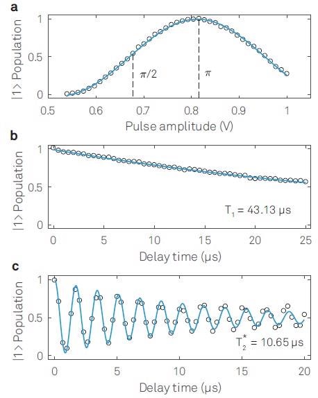
Figure 3. Single qubit characterizations: (a) Rabi-oscillation, (b) Qubit lifetime T₁ measurement and (c) Ramsey fringe measurement to extract .

Therefore, sweeping the amplitude within the pulse sequence helps in calibrating the pulse amplitudes required for the so-called π-pulse and π/2-pulse. While a π-pulse will bring the qubit precisely from the ground |0⟩ to its excited state |1⟩ akin to a logical inversion in traditional computing, the π/2-pulse will bring the qubit to an equal coherent superposition of both states.

It is important to characterize the lifetime of all four qubits because any decay from the excited to the ground state will restrict the gate performance. For this purpose, T₁—the qubit lifetime—is determined by bringing the qubit to its excited state with a π-pulse and then sweeping the delay until the qubit readout with the UHFQA Quantum Analyzer takes place. The resultant data, demonstrated in Figure 3 (b), is fitted to an exponential function exp(−T/T₁) in order to extract T₁ = 43.13 μs.

In a similar way, the qubit coherence time is calculated by a Ramsey experiment, by uploading the necessary pulse sequence to the HDAWG 1. It has two π/2-pulses segregated by a variable delay time followed by the qubit state readout. A further slight detuning of the pulse frequency in relation to the qubit frequency causes oscillations in the qubit population.

From the measurement illustrated in Figure 3, a of 10.65 μs can be obtained by fitting the signal with an exponential decaying cosine function.

The CPHASE Gate

The controlled phase (CPHASE) gate is one common method to implement a two-qubit gate, where the interaction between the |11⟩ and the two-photon energy level |20⟩ is exploited. [8] Furthermore, bringing these two levels on resonance will activate the CPHASE gate and a phase will be picked up by the second qubit based on the state of the control qubit. When a total phase of π is accrued, it means a logical inversion of the qubit’s state has occurred.

The so-called Chevron pattern has to be measured to characterize the length and amplitude of the flux-pulse which is required for such a gate operation. For this purpose, both qubits are initially prepared by applying one qubit gate on both (π_x-pulse). By changing the length and amplitude of a subsequent flux pulse on a single qubit, the gate operation is performed and the population exchanges coherently between the excited state |1⟩ and the ground |0⟩. Towards the end, the second qubit’s state is read out and compiled to the data plot, as illustrated in Figure 4.

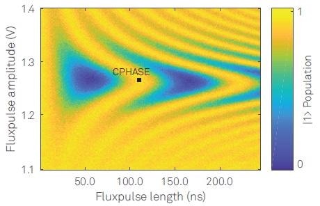
Figure 4. Chevron-Pattern of the CPHASE gate. A first π-pulse on both qubits is used to bring the system in the |11⟩ state and then a flux pulse with variable amplitude and length is applied, followed by the readout of qubit 2.

Now, the flux-pulse parameters can be calibrated for the CPHASE gate as denoted by the black marker shown in Figure 4, and the qubit-qubit coupling rate can be determined as an inverse of the required gate length. It must be noted that for this kind of experiment, the integrated HDAWG predistortion filter can be used to process the flux-pulse so as to offset the frequency dependent transmission via the flux-line.

The Bell State

The two-qubit gate performance is demonstrated by preparing a pair of adjacent qubits in a maximally entangled state, that is, a Bell state. Figure 5 (a) shows the sequence of gate operations needed.

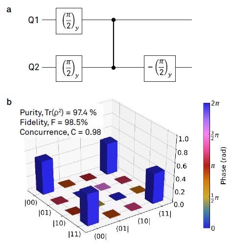
Figure 5. Bell state tomography: (a) Pulse Sequence for preparing the Bell state. The state was prepared with the aid of a CPHASE gate, illustrated by a vertical line. (b) Density matrix measured by state tomography. The obtained raw data was fitted with a Maximum-Likelihood estimation.

At first, both qubits are brought into an equal superposition by applying one qubit π/2-rotations. Both qubits are entangled by the next CPHASE gate operation and then the targeted Bell state (|00⟩+|11⟩)/√2 is obtained by a final qubit rotation.

Quantum state tomography is carried out to determine the density matrix ρ of the two-qubit system. [7] To obtain a physically meaningful result, the raw measurement data were fitted to a Maximum-Likelihood estimation. To compute the fidelity F of the state, the fitted data is compared to the ideal density matrix σ of the Bell state by assessing,

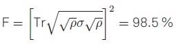(1)

A single-shot readout fidelity of F_R = 98.85% was considered in this calculation.

Outlook

The combination of UHFQAs and HDAWGs—ranging from important qubit characterizations to complicated multi-qubit gate operations—create an effective platform for quantum computing applications. A well-thought-out device synchronization concept will be needed to scale up to a higher number of qubits. The Programmable Quantum System Controller (PQSC) from Zurich Instruments not only eases this task but also facilitates the rapid development of large-scale quantum computing systems.

References

[1] M. Mohseni, P. Read, H. Neven, S. Boixo, V. Denchev, R. Babbush and A. Fowler, V. Smelyanskiy, and J. Martinis. Commercialize quantum technologies in five years. Nature Comment, 2017.

[2] S. M. Girvin, M. H. Devoret, and R. J. Schoelkopf. Circuit qed and engineering charge-based superconducting qubits. Physica Scripta,127:014012,2009.

[3] C. K. Andersen, A. Remm, S. Balasiu, S. Krinner, J. Heinsoo, J.-C. Besse, M. Gabureac, A. Wallraff, and C. Eichler. Entanglement stabilization using parity detection and real-time feedback in super-conducting circuits. arXiv:1902.06946v2[quant-ph], 2019.

[4] Zurich Instruments AG. Frequency up-conversion for arbitrary waveform generators.Technote, 2018.

[5] A. Wallraff, D.I. Schuster, A. Blais, L. Frunzio, R.-S. Huang, J. Majer, S. Kumar, S.M. Girvin, and R.J. Schoelkopf. Strong coupling of a single photon to a superconducting qubit using circuit quantum electrodynamics. Nature,431:1627,2004.

[6] M. D. Reed, L. DiCarlo, B. R. Johnson, L. Sun, D. I. Schuster, L. Frunzio, and R. J. Schoelkopf. High-fidelity readout in circuit quantum electro-dynamics using the Jaynes-Cummings nonlinearity. Physical Review Letters,105:173601, Oct 2010.

[7] J. Heinsoo, C. K. Andersen, A. Remm, S. Krinner, T. Walter, Y. Salathe, S. Gasperinetti, J.-C. Besse, A. Potocnik, C. Eichler, and A.Wallraf. Rapid high-fidelity multiplexed readout of superconducting qubits. Physical Review Applied, 2018.

[8] L. DiCarlo, M. Chow, J. M. Gambetta, Lev S. Bishop, B. R. Johnson, D. I. Schuster, J. Majer, A. Blais, L. Frunzio, S. M. Girvin, and R. J. Schoelkopf. Demonstration of two-qubit algorithms with a superconducting quantum processor. Nature, 460:240–244, 2009.

This information has been sourced, reviewed and adapted from materials provided by Zurich Instruments AG.

For more information on this source, please visit Zurich Instruments AG.