The Principles of Phase-Locked Loops in Analog Signals

Phase-locked loops (PLLs) for analog signals are a common feature in today's physics and engineering applications. This article presents the fundamental functions and operating principles of PLLs, as well as several practical use cases that can be easily implemented with Zurich Instruments' lock-in amplifiers.

Video credit: Zurich Instruments

The earliest PLL systems were proposed for the receivers of amplitude-modulated (AM) signals to take advantage of homodyne detection and to avoid the undesired image response caused by heterodyne receivers.¹

For proper operation, a homodyne detector requires a local oscillator (LO) with a frequency equal to the carrier frequency of the received signal. This means the LO must closely follow the phase of the incoming carrier. A PLL circuit was subsequently developed to lock the LO phase to the carrier phase, ensuring a constant or time-invariant phase relationship between the two oscillatory signals.

A PLL is a closed-loop control system with negative feedback, which maintains a well-defined phase relationship between two periodic signals - the input serves as a reference, while the output acts as a follower.

As a result of phase-locking, the two signals have the same frequency, which enables coherent signal generation and detection across multiple signal sources. In its simplest form, a PLL consists of the following building blocks²:

1. Phase detector
2. PID controller
3. Controlled oscillator

A PLL, as shown in Figure 1, receives an input signal from a reference source and transfers its phase evolution to a controlled oscillator to generate an output signal that follows the input signal's phase. The phase detector unit measures the phase difference between the two signals.

This difference is then compared to a set phase, known as the setpoint, to generate an error signal for the proportional-integral-derivative (PID) controller. Based on this error signal, the PID controller produces a feedback signal to adjust the frequency of the controlled oscillator. The controlled oscillator follows the input signal's phase and generates a signal at the same frequency as the input reference.

This white paper delves deeper into the building blocks of a PLL and explores the various applications of PLLs and the variations in their implementation based on the basic PLL scheme depicted in Figure 1.

It also provides useful tips on setting up a PLL, selecting its key parameters, and optimizing and characterizing its performance. The paper concludes with a summary of the different noise characteristics and models for PLL systems.

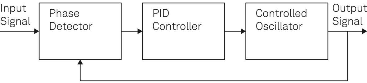
Figure 1. Schematic diagram of a PLL showing its basic building blocks. The PLL generates an output signal that follows the phase and frequency of its input signal. It is implemented using a negative-feedback closed loop. Image Credit: Zurich Instruments AG

PLL Building Blocks

PLL systems are designed to handle analog and digital signals depending on their intended application. This paper focuses on digitally implemented PLLs used for analog signals in advanced research and development experiments. The discussion centers on the use of digital signal processing for the implementation of phase detectors, PID controllers, and reference or controlled oscillators.

In particular, the focus of this paper is on Zurich Instruments’ PLLs. These PLLs utilize a field-programmable gate array (FPGA) to connect with analog input and output signals via analog-to-digital converters (ADCs) and digital-to-analog converters (DACs), respectively.

Phase Detector

A phase detector takes two periodic signals as inputs and generates an output signal proportional to the relative phase difference between the two input signals. Different techniques are employed for phase detection, depending on the signals used.

When dealing with square waves commonly used in digital systems, a phase detector is implemented using an XOR gate followed by a low-pass filter.³ More generally, dual-phase demodulation is used to obtain the phase difference by measuring the quadrature components X and Y of one input with respect to the other, as illustrated in Figure 2.

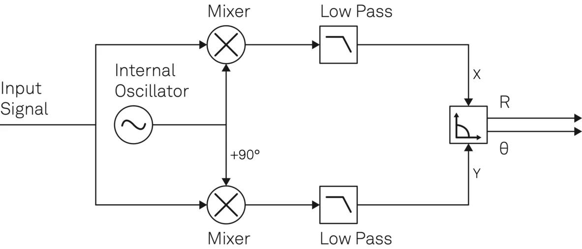
Figure 2. Phase detection using dual-phase demodulation of a lock-in amplifier. The in-phase component X and quadrature component Y are generated with two separate signal pathways to derive the relative phase θ and the signal magnitude R of the input signal. The low-pass filters can help to suppress unwanted frequency components and noise. Image Credit: Zurich Instruments AG

One of the most widely used instruments for dual-phase demodulation is the lock-in amplifier. These devices offer the added benefit of noise reduction and the ability to tune the PLL bandwidth, as seen in Figure 2. Low-pass filters can help to clean the input signal applied to the PID controller of undesired spectral components and noise present in either phase detector signal input.

These filters' cut-off frequency and phase delay set an upper limit on the overall PLL bandwidth.

Lock-in amplifiers for phase detection also have the added benefit of measuring the signal amplitude. This can be used for other control mechanisms, such as automatic gain control (AGC).

The amplitude R and the phase θ can be easily derived from the measured in-phase X and quadrature Y through a transformation from Cartesian to polar coordinates.

Equation 1

 

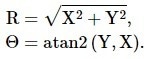
To accurately measure the phase difference between two input signals, it is important to use the correct method for phase detection. Using the 'atan2' function instead of ‘atan’ is particularly useful for this purpose, as it ensures that the phase angle covers all four quadrants of the phase circle, that is (−π, π], regardless of the sign of the quadrature components, as illustrated in Figure 3.

The discontinuity encountered while crossing quadrants may be readily identified and rectified in the digital realm when the phase signal varies slowly enough compared to the system's sampling rate.

This process is known as 'phase unwrapping', and it expands the range of phase values to many multiples of the original interval, as shown in the panels of Figure 4. Zurich Instruments’ lock-in amplifiers can support a wide phase capture range of up to ± 1024 π, which is necessary for applications such as stabilizing an optical interferometer over multiple wavelengths.⁶

Figure 3. (a) Polar coordinates illustrating the phase of a signal component pair (x,y) that covers a range from -180° to +180° represented by atan2(y,x). (b) Depending on the sign of x, atan2(y,x) is a double-valued function versus the ratio y/x returning the angle between the line to the point (x,y) and the positive x axis. Image Credit: Zurich Instruments AG

Figure 4. (a) Phase measured by a lock-in amplifier used as a phase detector. (b) Unwrapped phase demonstrating a linear relation between the actual and measured phase. Image Credit: Zurich Instruments AG

PID Controller

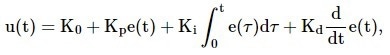
To create the error signal e(t), the PID controller accepts the phase difference output from the phase detector and deducts it from the user-defined setpoint. The error signal is then used to create feedback to the controlled oscillator using proportional, integral, and derivative procedures, as shown in Figure 5. As a result, the following equation gives the final feedback signal u(t):

Equation 2

 

where K₀ is the offset value and K_p, K_i, and K_d are P, I, and D coefficients, respectively. In many practical applications, utilizing the proportional (P) and integral (I) components results in a sufficiently well-performing and stable operation.

The derivative term can be incorporated to further decrease the mean deviation of the error signal from zero. However, it is important to note that the implementation of this term can introduce instability to the loop by amplifying high-frequency components of the error signal.

To mitigate this, an additional low-pass filter can be utilized, which suppresses the gain of higher frequencies, allowing for stable operation. It is important to note that the bandwidth of the closed-loop system characterizes the speed of the phase-locked loop (PLL).

When determining the appropriate control-loop bandwidth, it is important to consider the following factors:

1. Minimizing the average deviation of the error signal from zero typically requires optimization of the PID parameters to maximize the feedback bandwidth and gain. This approach is often effective in situations where large spontaneous disturbances are infrequent. In such settings, it leads to a settling time close to its minimum. To aid users in finding the optimal working point, Zurich Instruments PLLs come equipped with an Autotune functionality.
2. In some cases, high stability and a large capture range for the closed-loop operation may be of greater importance than minimizing the mean deviation of the error signal from zero. To achieve robustness against various types of external disturbances, it may be necessary to use a weaker and slower feedback signal, which reduces overreaction and prevents loss of control. This approach often results in a more robust start for the loop filter when initial conditions are not ideal. However, it is important to note that the optimal settings depend heavily on the specifics of the setup and may require manual tuning.

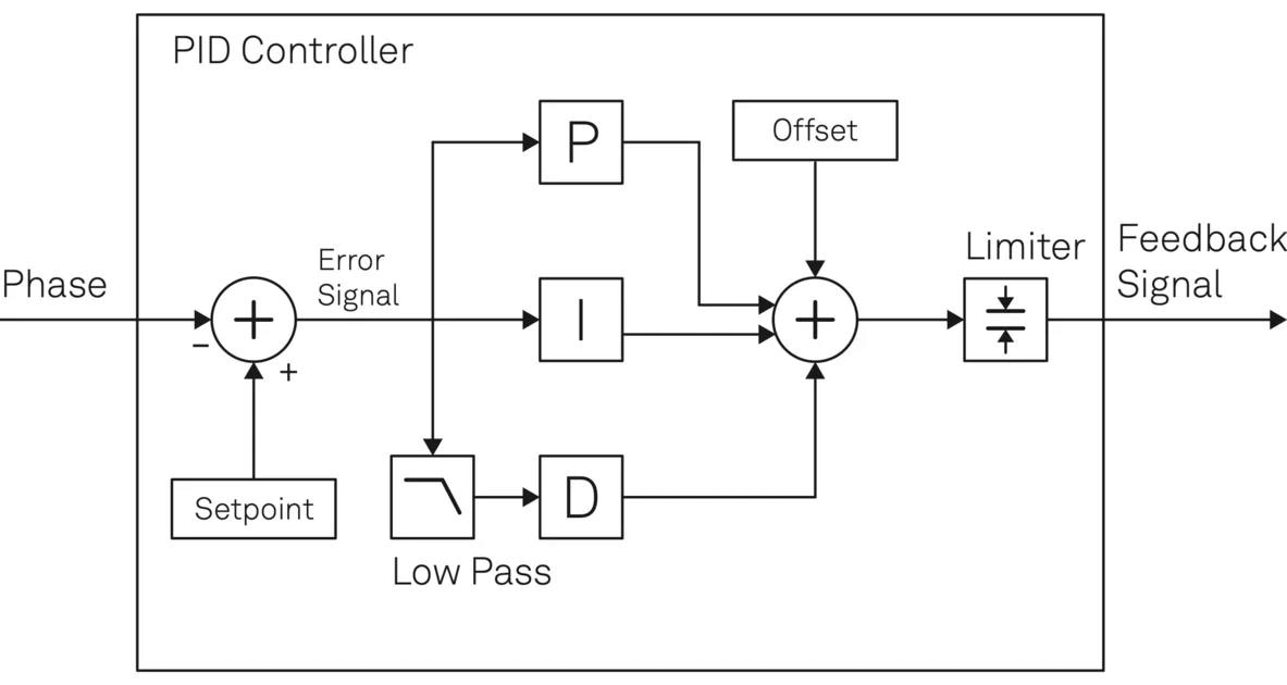
Figure 5. Schematic diagram of a PID controller: the phase signal from the phase detector is subtracted from the adjustable phase setpoint and the outcome then passes through the three different branches P, I and D before the resulting signals are added to an offset. A limiter helps restrict the range to a useful parameter space. Image Credit: Zurich Instruments AG

3. The input signal's noise components within the loop-filter bandwidth are the only ones transferred to the controlled oscillator. As a result, it is imperative to establish a clearly defined filter bandwidth. The utilization of powerful filtering enables the exclusion of unwanted frequency components from the output signal. Zurich Instruments' PLLs feature a PID Advisor, which models all components involved in the loop and aids users in identifying and setting up the necessary bandwidth promptly.

An additional feature of significant practical relevance is the adjustable output offset, which enables starting from a default position of the PID controller output, providing users with a beneficial starting point when the loop is activated. The capability to set upper and lower limits for the feedback signal enables the restriction of the control operation to a user-defined frequency range.

This is particularly useful when the input signal contains multiple distinct frequency components, but only one needs to be tracked, or when preventing damage to external equipment is a concern. 

Oscillators and Frequency References

The controlled oscillator in a PLL can be realized through either a voltage-controlled oscillator (VCO) or a numerically controlled oscillator (NCO), as they both allow for frequency adjustments through analog and digital feedback, respectively.⁷

VCOs are commonly utilized as externally controlled oscillators and are widely available active components that emit a sinusoidal signal with a fixed amplitude. Their frequency can be varied within a specific range using an analog input voltage. The main feature of a VCO is the degree to which its frequency changes about the control voltage, which ideally follows a linear relationship.

On the other hand, NCOs always assure linearity and provide the added benefit of having frequency values that are digitally available at any given time, also functioning as a frequency counter. While there are several methods to produce controllable periodic signals, most instances can be traced back to either a VCO or NCO regarding basic functionality.

An example of this can be seen in the beat note between a laser beam and a frequency comb, which typically creates a radio frequency signal at the output of a photodiode. By applying a feedback signal to the modulation input of the laser, its optical frequency will change in accordance with the voltage signal, resulting in a change in the frequency detected by the photodiode.

This is similar to using a VCO and can be utilized, for instance, to establish an optical PLL for laser frequency stabilization.

When using Zurich Instruments' Lock-in Amplifiers, one input to the phase detector always comes from an internal digital oscillator. The frequency of these NCOs, which are implemented on an FPGA, can be adjusted digitally while maintaining a steady phase continuous output.

The rate at which the NCO frequency can be altered is determined by either the FPGA clock speed or the frequency register update rate. This rate is significantly higher than the maximum achievable control-loop bandwidth.

Depending on the PLL configuration, the internal NCO can serve as a leader, a follower, or an intermediate oscillator. If the NCO follows an external frequency reference, the internal NCO's frequency is adjusted numerically by the PID controller to keep pace with the reference signal.

However, if the internal oscillator provides the frequency reference for an external VCO, its frequency is fixed at a specific value while the PID controller adjusts the frequency of the external VCO through feedback. In situations where two external sources must be locked, two PLLs must be set up with a shared internal NCO serving as an intermediate transmission gear.

It is noteworthy that generating accurate and precise periodic signals within a wide frequency range is crucial for various test and measurement (T&M) applications. Many T&M instruments that cover a broad frequency range use PLL-based frequency synthesis to generate adjustable periodic signals.

PLLs can combine the flexibility of wide-range and precise frequency generation with high stability and accuracy by integrating the best properties of highly accurate and low phase-noise oscillators, such as oven-controlled crystal oscillators (OCXO), with the flexibility of controlled oscillators, such as VCOs. A PLL synchronizes the controlled oscillator frequency f with a fraction of the OCXO frequency f_REF, which serves as a reference.

Adjusting the coefficient factor, a wide frequency range according to f = (m/n) f_REF, as seen in Figure 6, is achievable. The oscillator frequency can now be widely tuned by numerically adjusting the ratio m/n. In contrast, the OCXO frequency remains fixed at a stable frequency, such as 10 or 100 MHz, in many T&M instruments.

In addition to frequency accuracy and stability, the implementation details of the PLL also affect other factors such as phase noise, spur sidebands, and lock-time, all of which determine the quality of the generated signal and ultimately influence the performance of systems in which such frequency synthesis is implemented.

For most digital signal processing instruments, this functionality is built-in. Therefore, the signal of the internal NCOs serves as a reliable frequency reference.

Applications

The primary function of a phase-locked loop is to synchronize two systems in terms of time, primarily through two oscillators. There are numerous applications where the synchronization of two or more oscillatory signals is necessary.

While PLLs are commonly used in digital systems for tasks such as jitter reduction, skew suppression, frequency synthesis, and clock recovery, this discussion will focus on the applications of PLLs for analog signals, specifically those that fall under one of the following three configurations:

1. Frequency tracking: the PLL maps an external source to an internal oscillator, see Figure 6.
2. Resonance driving: the PLL drives the time-varying resonance of a device, see Figure 9.
3. Oscillator control: the PLL provides analog feedback to an external variable-frequency source, see Figure 10.

Frequency Tracking

A wide range of applications, such as lock-in amplifiers, transmission systems, and embedded systems, require coherent signal detection, which necessitates synchronizing the signal source and the signal detector.

In its most general form, as illustrated in Figure 6, a frequency tracking system receives an external reference signal and maps its frequency content to the internal oscillator of the system. A concrete example of this application is homodyne detection by a lock-in amplifier with an external reference.

To effectively recover the amplitude and phase of an input signal, a lock-in amplifier needs an external reference signal from the signal generator, which determines the measurement frequency, such as an optical chopper. The lock-in amplifier then needs to synchronize its internal oscillator to that external reference frequency to detect the received signal of interest coherently.

This is typically done through a PLL configuration similar to Figure 6. Finding the appropriate center frequency and bandwidth of the PLL is usually automated for most use cases. However, when specific bandwidth requirements are given or the spectrum contains multiple components, adjusting individual PLL settings may be necessary to ensure accurate frequency tracking.

This mapping of an external reference signal to an internal oscillator by using a defined bandwidth results in a jitter- and spurious-free signal at the tracked frequency. This can be beneficial for applications that require spectral filtering, as one can choose a deliberately low closed-loop bandwidth to exclude or suppress unwanted noise sources of the external signal.

Another benefit of an all-digital implementation is the ability to multiply or divide the tracked frequency to generate an internal reference at its harmonics and ratios without any loss of signal quality.

Using fractional multiples of the reference frequency for demodulation enables additional measurement schemes based on the same external reference, for example, optical chopping with harmonic-blade wheels.

Another significant application of the PLL configuration in Figure 6 is carrier recovery. Coherent demodulation of received signals in a transmission system requires the receiver to be aware of the frequency of the carrier wave.

However, due to the distance between the transmitter and receiver, they cannot share the same clock source. Perfect synchronization is unattainable unless the receiver uses a PLL to lock to the carrier sent by the transmitter. In addition to the modulated signal, many communication systems send a pure tone as a pilot to which the receiver's PLL can lock.

Without carrier recovery by a PLL unit, coherent communication cannot be achieved in most transceiver systems. In situations where no pilot is sent, or the modulated signal is carrier-suppressed, slightly modified PLL configurations, such as Costas loops, are utilized to extract the carrier frequency.⁸

Similarly, for lock-in amplifiers, when a distinct external reference is not available, it may be possible to lock the internal oscillator to the measurement signal itself, depending on the signal quality. This so-called 'auto-reference' configuration of lock-in amplifiers can only extract the amplitude information of the signal and not the phase.

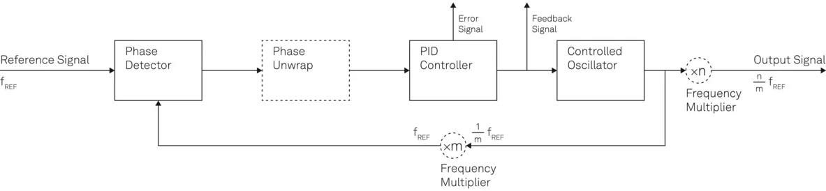
Figure 6. Schematic diagram showing the building blocks of a PLL with extended functionality for phase unwrap and fractional frequency locking. Besides the output signal, many applications benefit from intermediate signals such as error and feedback signals. Image Credit: Zurich Instruments AG 

Frequency Extraction, Filtering and Counting

PLLs can extract specific frequency components from signals that contain multiple distinct frequencies. This process requires fine-tuning the variable source to the desired frequency before the PLL start-up to transfer the targeted spectral component to the internal oscillator of the PLL.

This technique is highly versatile and can filter out specific spectral components, track them, and utilize them as pure signals in other parts of the setup. Because the feedback to the internal NCO is digital, the instantaneous frequency can be tracked and recorded at a high rate, providing additional frequency-counting functionality.

FM Demodulation

Frequency modulation (FM) is a method of encoding information from a message signal into the frequency of a carrier wave. It is widely used in analog and digital systems due to its resistance to changes in amplitude and noise.

In FM systems, the instantaneous frequency of the carrier changes in accordance with the time variation of the message signal. Therefore, a device that can track the frequency is necessary to demodulate the carrier wave and extract the message from the carrier frequency. Among the different techniques for demodulating FM systems, the PLL is particularly effective due to its low distortion levels and reduced sensitivity to amplitude noise.

A PLL-based FM demodulator is a relatively simple process and does not require significant changes to the basic PLL configuration, as depicted in Figure 7. When no modulation is applied to the carrier wave, the feedback signal applied to the controlled oscillator is set to generate the carrier frequency.

However, when the modulation changes the carrier frequency, the loop filter adjusts the feedback voltage applied to the oscillator to change its frequency. This way, the closed loop remains locked, meaning that the oscillator signal follows the phase of the received FM signal. The feedback signal applied to the controlled oscillator is proportional to the frequency change of the received carrier.

The demodulated signal can be amplified and sent to the next stage for acquisition and processing.

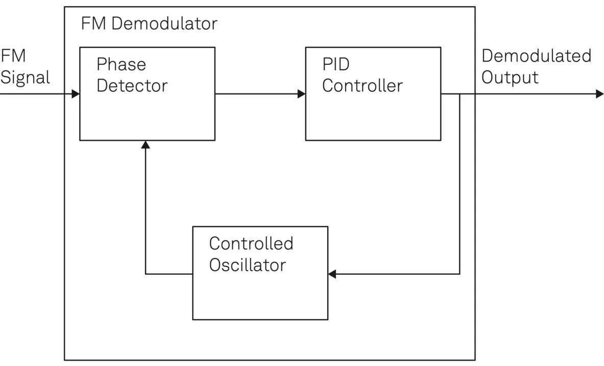
Figure 7. Schematic diagram of a PLL-based FM demodulator where the output of demodulation is proportional to the feedback signal applied to the controlled oscillator. Image Credit: Zurich Instruments AG

The main consideration in designing a PLL-based FM demodulator is the demodulation bandwidth, which is determined by the PLL's closed-loop bandwidth. The demodulation bandwidth determines the signal bandwidth and the maximum amount of information transmitted over the communication channel per time.

Therefore, the phase detector and PID controller must be fast enough to cover the required bandwidth of the FM signal. Using an oscillator with a highly linear response is crucial to minimize distortion of the demodulated signal and keep the demodulation process as linear as possible.

When using VCOs as controlled oscillators, the voltage-to-frequency curve must be as linear as possible within the frequency range of the received FM signal.

Resonance Driving

Driving a device with a controlled phase and frequency is essential in various applications such as atomic force microscopy (AFM) and micro- and nano-electromechanical systems (MEMS/NEMS).

These systems often behave like a resonator with a Lorentzian-shaped amplitude transfer function and a sigmoid-shaped phase evolution, as illustrated in Figure 8, which shows the Bode magnitude and phase plots of a resonator with a resonance frequency of 1.84 MHz.

To benefit from resonance enhancement and linearization of the measurement response, it is crucial to driving the device at its resonance frequency. However, the resonance frequency of such systems often varies with environmental factors such as temperature and force. To maintain a fixed phase, the drive frequency must be adjusted accordingly.

A PLL-controlled resonator drive, as shown in Figure 9, can achieve this by continuously adjusting the drive frequency in response to changes in the resonator's resonance frequency.

The PLL utilizes a phase detector to compare the phase of the drive signal and the resonator's output, and a PID controller to adjust the frequency of the drive signal accordingly. This ensures that the device is always driven at the same working point, even when the resonance frequency changes over time.

The cantilever head of an Atomic Force Microscope (AFM) features a tuning-fork resonator, which measures the force field exerted on the surface of the sample under examination by way of the induced shift in its resonance frequency.

To measure this frequency shift and, as a result, characterize the surface topography, a Phase-Locked Loop (PLL) is required to lock onto the cantilever's resonance. The PLL error signal will then represent the sample surface.

Another typical example of applying PLLs can be found in inertial measurement systems, such as Micro-Electro-Mechanical Systems (MEMS) gyroscopes and accelerometers.⁵ It is crucial to driving the vibrational mass of such systems at their resonance frequency, regardless of the rotational motion they observe. Since rotation alters the resonance frequency, a PLL is essential for the stable drive of the sensor at its varying resonance frequency.

This application of PLLs in controlling resonance systems includes various examples, such as pump-probe, ion trapping, and parametric feedback cooling experiments. In these cases, the PLL is modified to adapt to the application-specific requirements. For example, in parametric feedback cooling, the system is driven out-of-phase at the second harmonic of the resonance frequency.⁹

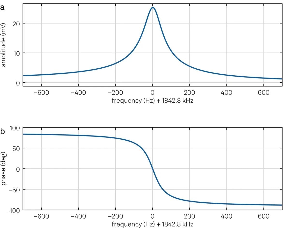
Figure 8. (a) Bode magnitude and (b) phase plots of a crystal resonator measured by the frequency response analyzer of a Zurich Instruments lock-in amplifier. Image Credit: Zurich Instruments AG

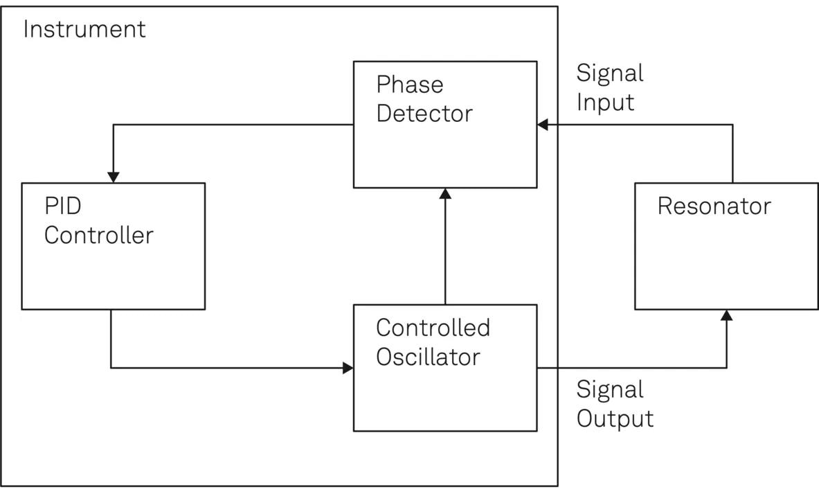
Figure 9. Schematic diagram showing the closed-loop control of a resonator by means of a PLL. The resonator together with the instrument form a PLL system where the controlled oscillator follows the varying resonance frequency by keeping the relative phase constant. Image Credit: Zurich Instruments AG 

Oscillator Control

As previously mentioned, and for the sake of simplicity, any external oscillator to be controlled is modeled as a Voltage-Controlled Oscillator (VCO). In the Phase-Locked Loop (PLL) configuration illustrated in Figure 10, the internal oscillator provides the reference signal for the phase detector, which measures the phase of the external oscillator relative to the reference.

The Proportional-Integral-Derivative (PID) controller converts the measured phase difference into a feedback signal and applies it to the external VCO to adjust its output frequency. This enables the mapping of the time-based content of a stable internal Numerically-Controlled Oscillator (NCO) to an external system.

The spectral filtering of the phase detector, in conjunction with the programmable output limiter of the analog voltage signal, contributes to stable operation at the desired frequency, even after re-locking if the lock is lost. The system is not driven at any values outside the defined safe zone, where reliable operation is guaranteed even if the integrator goes into saturation.

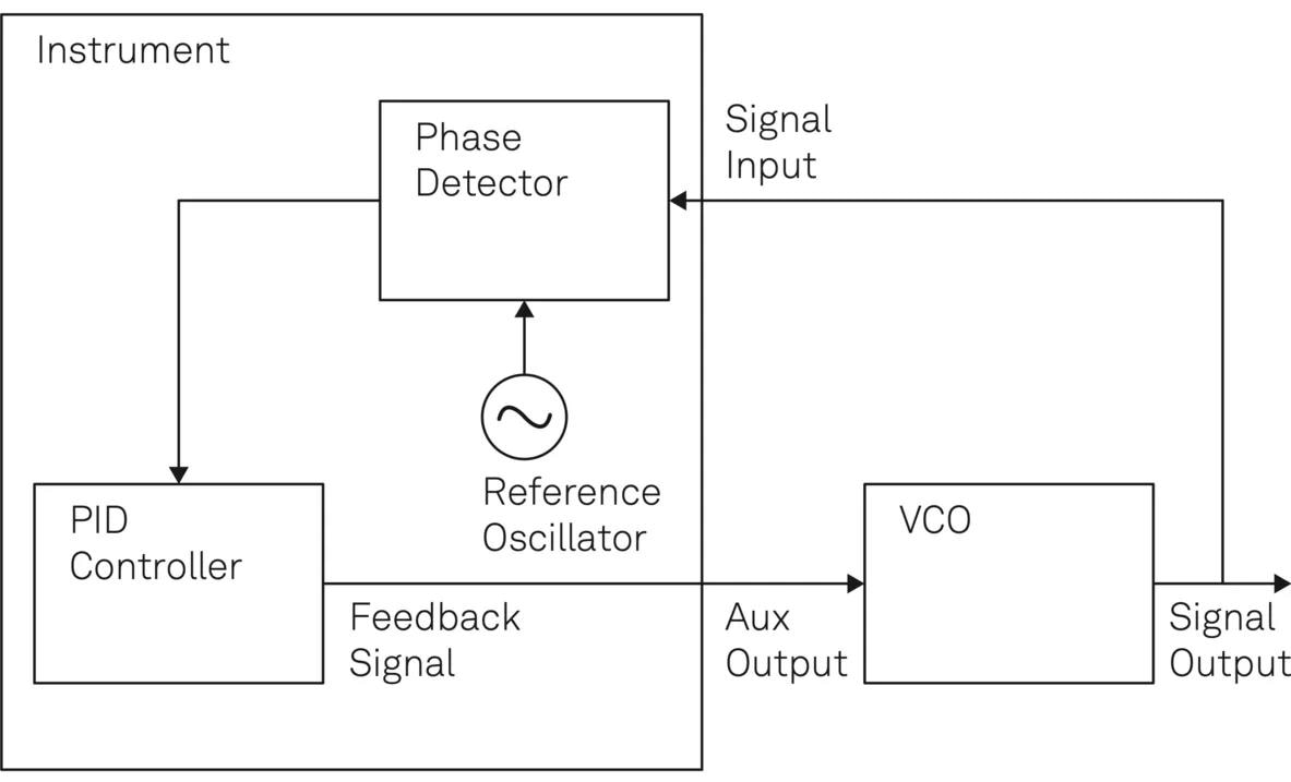
Figure 10. Controlling the frequency of a VCO based on a reference oscillator using a phase-locked loop. Image Credit: Zurich Instruments AG 

Starting up a PLL

The following steps describe a systematic process for successfully closing a feedback loop and getting a PLL operating:

1. Obtain the open-loop response of the system
2. Find a coarse and conservative set of PID parameters to start the loop
3. Tune the PID parameters to optimize for SNR, speed, or robustness

Finding an appropriate initial set of Proportional-Integral-Derivative (PID) parameters and starting conditions can be a challenging task. LabOne^®, the Zurich Instruments control software that interfaces with the instrument hardware, provides effective tools to make the time-consuming process of starting up and optimizing a Phase-Locked Loop (PLL) as efficient and easy as possible.

As a first step, obtaining the open-loop response of the Device Under Test (DUT) is necessary. This can be the spectral response of a resonator or the curve displaying the frequency with respect to the tuning voltage of a Voltage-Controlled Oscillator (VCO).

The sweeper module of LabOne offers all the necessary tools to obtain the open-loop response of a system, as it can sweep the frequency, phase, amplitude, and offset of the applied signals, and acquire the measured outcome.

The integrated mathematical tools, such as curve fitting, tracking, peak-trough finding, etc., help the user extract the system characteristics, such as quality factor, gain, and slope, needed for proper PID controller tuning.

Determining the appropriate target bandwidth for a Phase-Locked Loop (PLL) system can be achieved by taking into account various factors, such as the characteristics of the low-pass filter used in the phase detector unit and the system delays introduced at various points.

To facilitate this process, LabOne^® offers a convenient PID Advisor tool. This tool employs an optimization algorithm to tune the Proportional-Integral-Derivative (PID) controller and determine the required filter settings for a given target PLL bandwidth.

The PID Advisor takes into account all physical delays and gains of the hardware and provides a variety of mathematical models to factor in the transfer function of the attached device. Once the device configuration is selected, the Advisor runs its algorithm to calculate the P, I, and D parameters and obtains the filter characteristics, phase margin and actual bandwidth.

The tool provides various temporal and spectral figures, such as Bode magnitude and phase plots, plus the step response at various entry points of the entire system, to illustrate the performance of the designed PLL in terms of stability and speed. This makes starting up and optimizing a PLL system more efficient and straightforward.

The application of PID settings obtained through the use of the PID Advisor to the instrument, along with the enabling of the PID controller, should result in the successful closing of the PLL. Using the plotter tool within LabOne allows for continuous monitoring of the PID error and output signals. This allows for adjustments to be made to the PID settings while observing the impact on the performance of the PLL.

In addition to the manual adjustment of PID parameters, the Autotune feature of the PID controller, available within LabOne, can also be utilized to modify the PID settings automatically to improve the performance of the PLL. Figure 11 illustrates the PID/PLL tab within the LabOne user interface, providing all necessary tools for designing, optimizing, and running a PLL within a user-friendly web environment.

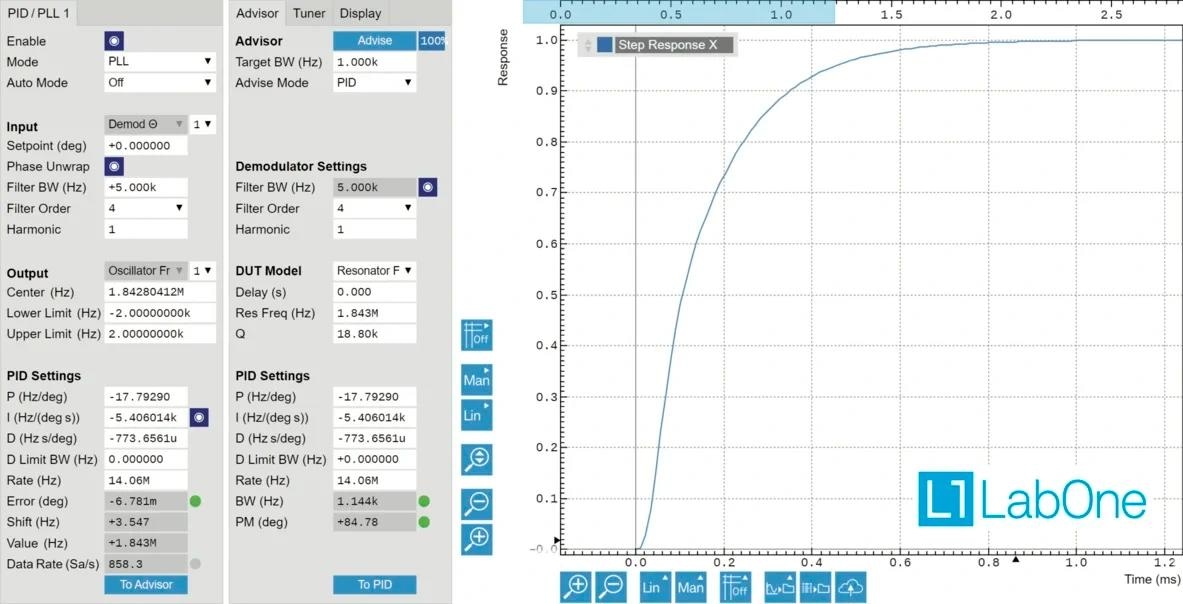
Figure 11. PLL/PID controller tab of LabOne user interface showing the input, output, phase unwrap, and PID parameters (left), PID Advisor, Tuner, and DUT model (middle), and the step response of the final closed-loop system (right). Image Credit: Zurich Instruments AG

Noise in PLLs

The analog output of a PLL is typically a sinusoidal signal characterized by a fixed amplitude but a varying frequency and phase that is synchronized to a setpoint or reference signal.

In an ideal PLL, the frequency and phase of the output signal should remain constant over time. However, in practical systems, noise can cause fluctuations in both the frequency and phase of the output signal.

The phase fluctuation can be modeled as a zero-mean random process, represented by φ(t), with a standard deviation of σ_φ. Therefore, the output of a PLL with a fixed setpoint can be represented by the following sine signal, where the carrier frequency is denoted by f_c in Hz and the phase is represented by ψ in rad:

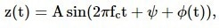Equation 3

 

where A is a fixed amplitude. The phase noise, which is inherent in any PLL system, is best represented by its power spectral density (PSD), denoted by S_φ(f). This is obtained by taking the Fourier transform of the auto-correlation of φ(t). The PSD represents how much noise power exists in a unit bandwidth of 1 Hz at an offset frequency f away from the carrier frequency fc. Its unit is rad²/Hz. However, in many applications, it is also expressed in dBc/Hz, relative to the carrier power.

The IEEE standard defines S_φ(f) in rad²/Hz as the one-sided (double sideband or DSB) spectral density of phase and introduces the two-sided (single sideband or SSB) spectral density L_φ(f) as a standard way of representing phase noise in dBc/Hz.

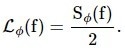Equation 4

 

It is important to note that the phase noise PSD provided in data sheets is always 3 dB below the actual one-sided spectrum. Care should be taken when calculating the noise power and temporal jitter based on spectral density (citation). In other words, the phase noise power σ_φ² within a measurement bandwidth δf, expressed in rad², can be obtained by either of the following two integrals:

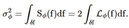Equation 5

 

For instance, a PLL with a constant SSB phase noise of −120 dBc/Hz around a specific offset frequency suffers from a phase fluctuation of  μrad caused by a 5-Hz measurement bandwidth around that particular offset frequency.

It is important to note that according to the fundamental relationship between frequency and phase, the frequency fluctuation ν(t) of the PLL output in Hz can be obtained from its phase noise using the following expression:

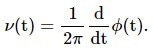Equation 6

 

Similarly to the phase noise PSD, the power spectral density of frequency noise can also be defined as the Fourier transform of its auto-correlation (citation). The frequency noise PSD, denoted by S_ν(f), is expressed in Hz²/Hz, and it can be obtained from the phase noise PSD using the following equation:

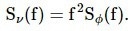Equation 7

 

Depending on the specific application, it may be important to focus on either the phase noise or the frequency noise of a PLL system. Equation 7, previously mentioned, provides a means for converting the power spectral density (PSD) of one type of noise into that of the other. 

Power Law

A power-law function is used as a heuristic way to represent the power spectral density of phase and frequency noise:¹¹

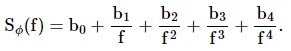Equation 8

 

The above expression denotes various types of noise, each represented by a distinct term. For example, the term b₁ represents the contribution of flicker phase noise to the spectral density, characterized by a slope of -10 dB/decade. Similarly, the term b₂ corresponds to Brownian phase noise, which exhibits a slope of -20 dB/decade within the noise spectrum. As per Eq. 7, the frequency noise spectrum can be described utilizing a power-law function.

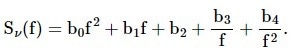Equation 9

 

Table 1 illustrates the various colors of phase and frequency noise that contribute to the overall noise spectral density of a Phase-Locked Loop (PLL) system. Each color corresponds to a specific slope on a logarithmic scale within the spectrum. Specifically, the term "fi" in the table represents a noise color that exhibits a slope of 10i dB/decade in the spectral density.

Figures 12 and 13 depict the phase and frequency noise spectrum of an oscillator controlled by a PLL. Depending on the components of the PLL system, certain noise colors may dominate within a specific frequency range, as observed by the slope of the spectrum curve in that range.

For instance, in the case depicted in Figure 12, the phase noise is almost white for frequencies above 1 kHz, as the spectrum curve is relatively flat within this range. It should also be noted that the power-law description of phase noise is closely related to the Allan variance or the Allan deviation, which are time-domain tools used to analyze the noise characteristics of an oscillator.

The other parameter can be acquired by measuring the spectrum or the Allan variance and providing a detailed description of phase and frequency noise in the time and frequency domains.¹¹

Table 1. Various types of phase and frequency noise and their contribution to the noise spectrum. Credit: Zurich Instruments AG

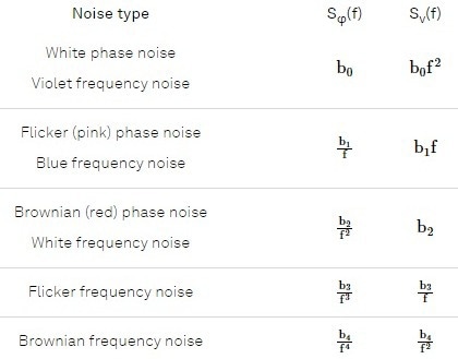
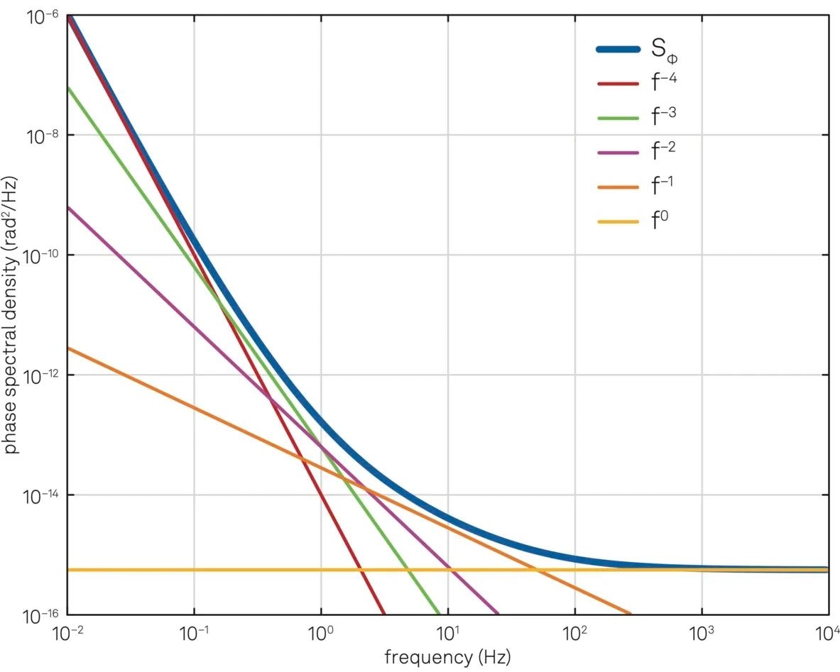
Figure 12. Phase noise spectral density and the contribution of different noise colors. Image Credit: Zurich Instruments AG

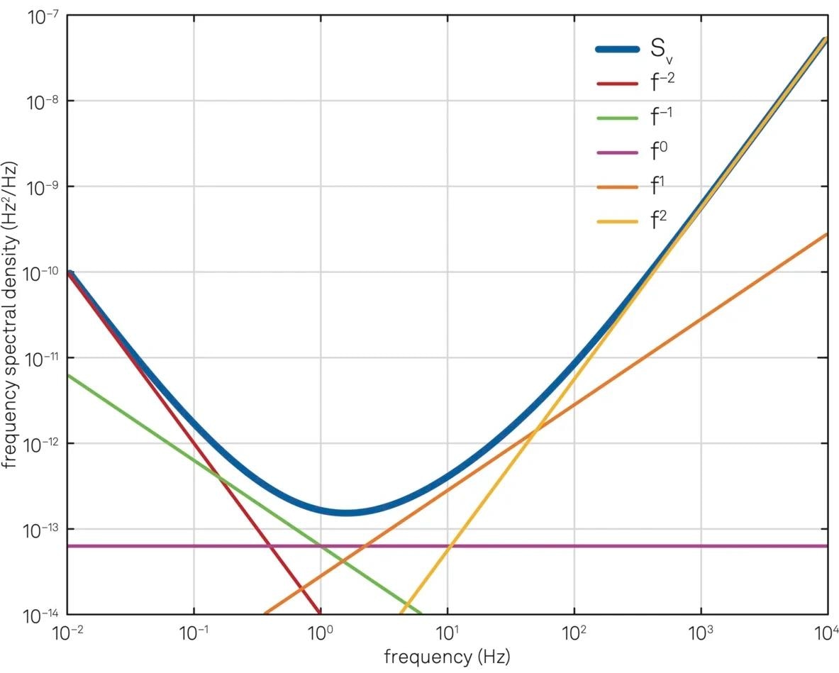
Figure 13. Frequency noise spectral density and the contribution of different noise colors. Image Credit: Zurich Instruments AG 

Leeson Effect

A typical scenario in resonance tracking is one in which a resonator is driven by a Phase-Locked Loop (PLL) system, where the white phase noise of the VCO is the dominant noise source. Under these circumstances, it is expected that the frequency noise will have an order of f².

However, in addition to this violet frequency noise, a white frequency noise term may also be present. This can be attributed to the Leeson effect.¹²

According to the Leeson effect, the phase noise S_φ at the output of the resonator can be derived from the VCO phase noise S_ψ at the input of the resonator by the following expression:¹¹

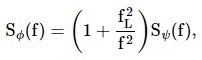Equation 10

 

where f_L =f₀/2Q is referred to as the Leeson frequency. If the VCO has a white phase noise of b0, then according to Equation 10, the phase noise of the resonator includes a white term b0 and a red term b₀f_L²/f².

Applying Equation 7 to the resonator phase noise leads to a frequency noise spectrum with two terms: a blue term b₀f² and a white term b₀f_L². Figure 14 illustrates the spectrum of the resonator's phase and frequency noise when driven by a VCO with white phase noise.

The figure clearly illustrates that for frequencies above the Leeson frequency of the resonator (in this case, f_L = 20 Hz), the dominant noise is from the VCO. Conversely, for frequencies below f_L, the resonator contributes to the noise spectrum and modifies the noise color.

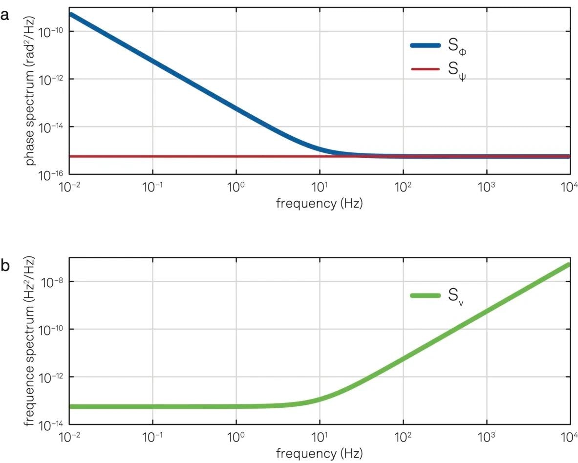
Figure 14. (a) Phase noise of a resonator (blue line) with a Leeson frequency of 20 Hz driven by a controlled oscillator with white phase noise (red line). (b) Frequency noise of the resonator. Image Credit: Zurich Instruments AG

Conclusion

Phase-locked loops are extensively utilized in physics, electronics, photonics, and communications as an important component for phase and frequency tracking and synchronization.

A phase detector, a PID controller, and a regulated oscillator are the three essential components of a PLL. Each of these building parts adds to the overall system reaction. The three major PLL designs may be used to achieve the most typical PLL applications: frequency tracking, resonance driving, and oscillator control.

Closed-loop frequency and phase control with integrated features such as phase unwrapping and autotune functionality, as well as user-friendly tools such as the PID Advisor and parametric sweeper, are provided by FPGA-based phase-locked loops for analog signals, such as those offered with Zurich Instruments' lock-in amplifiers.

References

1. Thomas H. Lee. The Design of CMOS Radio Frequency Integrated Circuits, 2nd ed. Cambridge University Press, 2003.
2. Roland E. Best. Phase-Locked Loops. McGraw Hill, 2003.
3. Behzad Razavi. Design of Analog CMOS Integrated Circuits. McGraw Hill, 2002.
4. Zurich Instruments. Principles of Lock-in Detection, 2016.
5. Zurich Instruments. Control of MEMS Coriolis Vibratory Gyroscopes, 2015.
6. Zurich Instruments. Interferometer Stabilization with Linear Phase Control Made Easy, 2018.
7. Donald R. Stephens. Phase-Locked Loops for Wireless Communications: Digital, Analog and Optical Implementations. Wiley, 2002.
8. J.P. Costas. Synchronous communications. Proceedings of the IEEE, 90(8):1461–1466, 2002.
9. Zurich Instruments. Parametric Feedback Cooling, 2014.
10. IEEE standard definitions of physical quantities for fundamental frequency and time metrology--random instabilities. IEEE Std. Std 1139-2008, 2009.
11. Enrico Rubiola. Phase Noise and Frequency Stability in Oscillators. Cambridge University Press, 2010.
12. D. B. Leeson. A simple model for feedback oscillator noise. Proceedings of the IEEE, 54(2), 1966. 

This information has been sourced, reviewed and adapted from materials provided by Zurich Instruments AG.

For more information on this source, please visit Zurich Instruments AG.